Master Thesis - Predictive Coding @ SILS

A full breakdown of my MSc Artificial Intelligence thesis, "Predictive Coding Graphs for bidirectional learning with local updates", conducted at the SILS lab (UvA, Cognitive and Systems Neuroscience). The work studies predictive coding (PC) as a biologically grounded alternative to backpropagation, generalized from hierarchical networks to arbitrary directed graphs, so that classification, generation, and occlusion/reconstruction all live inside a single model.

About this write-up: this is a detailed, long-form breakdown of the thesis, with the real figures and tables embedded throughout. The complete PDF is linked at the top of the page. An interactive implementation/demo may follow.

Abstract

We study predictive coding (PC) on arbitrary directed graphs, unifying classification, generation, and occlusion within one model. We evaluate hierarchical, fully connected, and stochastic block models (SBMs) on MNIST-scale tasks. We show that shallow PC models are competitive for classification, but deeper models amplify training instability and update divergence compared with traditional backpropagation (BP). Generative PC models querying via clamped labels yield plausible yet weakly controllable MNIST image samples and are sensitive to hyperparameters. Fully connected graphs favor shortcut credit paths that collapse into near direct (sensory–label) mappings, bypassing rich latent structure. In contrast, clustered sparse topologies discourage direct sensory-to-label bypasses and scale to larger node counts without degrading accuracy. Overall, PC is promising for parallel, local learning on sparse graphs, but remains limited by sensitivity to initialization, step sizes, and topology.

Keywords: predictive coding, inference-learning, graph topology

Motivation: why look past backpropagation?

Backpropagation (BP) has been essential to the success of deep learning, but its reliance on sequential backward passes, non-local computations, and acyclic architectures makes it biologically implausible. BP splits training into a forward pass (compute activations) and a backward pass (compute gradients and propagate errors), and there is no evidence of such a distinct reverse signaling phase in biological circuits. Biological learning instead appears local in space and time: neurons update based on nearby activity and plasticity rules rather than a single global objective, and the needed memory is carried by short-lived synaptic traces, not explicit neuron-level caches stored after the forward pass.

Predictive coding offers a different bargain. It performs inference and learning in a unified process without a dedicated backward pass: it continually updates neuron activities to minimize prediction errors, and weight updates follow from those same local errors. The standard PC learning algorithm, often called Inference Learning (IL), does not store or reuse the original feedforward activations to compute weight updates, unlike BP, which must cache them. PC networks (PCNs) can also act as classifiers, generators, and associative memories within a single framework, and recent work has adapted them to arbitrary graph topologies. Building on the arbitrary-graph formulation of Salvatori et al. and the hierarchical implementation of van Zwol et al., this thesis implements PCNs on arbitrary graphs to unify classification, generation, and associative memory in one model, and compares hierarchical, fully connected, and stochastic-block topologies.

Figure 1: Locality contrast between BP and PC — Figure 1: Locality contrast, BP propagates a global error through the network, whereas PC updates each synapse using only local activity and the prediction error of its directly connected postsynaptic neuron.

From a machine-learning standpoint, PC has promising properties: it achieves strong results in classification and memorization, has been shown competitive with BP on small datasets when using feedforward PC models, and a hierarchical PC implementation even reaches 99.9% accuracy on CIFAR-10. BP still holds the upper hand on larger datasets (e.g. CIFAR-100), where established tricks like BatchNorm, dropout, and robust optimizers give it a consistent edge, and where PC's instability, vanishing/exploding dynamics and sensitivity in recurrent or dense graphs, becomes costly.

Predictive coding background

PCNs were first introduced for unsupervised feature learning by Rao & Ballard (1999) and later extended to supervised learning. The core idea: the brain maintains an internal generative model that continuously predicts incoming sensory data; the discrepancies between predictions and actual inputs, the prediction errors, are used to update the internal model. Higher levels predict the activity of lower levels, all the way down to predicting direct sensory input. Given a clamped sensory stimulus, representations are updated using bottom-up prediction errors and passed as messages to higher layers, which in turn refine their own predictions. This is, mathematically, hierarchical variational Bayesian inference under a Gaussian posterior.

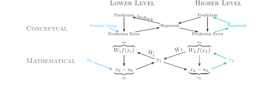
Figure 2: Hierarchical predictive coding framework — Figure 2: The hierarchical PC framework across lower and higher levels, in supervised learning the top representation x_L is clamped to the label corresponding to the sensory image x_0.

Each layer minimizes its own prediction error by comparing top-down predictions with bottom-up inputs; errors flow upward and refine internal representations until a stable representation is reached throughout the hierarchy. This bidirectional flow, bottom-up sensory inputs and top-down predictions interacting, is the engine of adaptive learning, and is fundamental to areas such as the hippocampus.

Energy, free energy, and the objective

Casting PC as Bayesian inference: given observations o (images or labels), we want to infer the latent states x that caused them, under a generative model p(o, x; θ) = p(o|x; θ)p(x; θ). The marginal likelihood is intractable, so we optimize a tractable bound, the variational free energy, equivalently the negative ELBO. The free energy decomposes as Complexity − Accuracy, trading off generalization against fitting the data:

F(x, o, θ) = KL[ q(x|o,θ) ‖ p(x|θ) ]  −  E_q [ log p(o|x,θ) ]
             \________ Complexity _______/   \____ Accuracy ____/

Assuming a hierarchical Gaussian generative model with unit covariance and a Laplace mean-field approximation, the negative log-likelihood collapses to squared prediction errors, recovering the original Rao & Ballard objective:

F(x, y, θ) = Σ_l ‖ x^(l) − µ^(l) ‖²  =  Σ_l ‖ ε^(l) ‖² ,   ε^(l) = x^(l) − µ^(l)

This establishes PC as energy-based inference arising from a Gaussian hierarchical model, jointly minimized over activities and parameters, and serves as the basis for extending PC to arbitrary topologies.

Inference Learning: the two-phase loop

The learning dynamics of many PC models can be read as an EM-like alternation that jointly minimizes the shared free energy F. The E-step (inference) infers the best causes (node activities) given fixed parameters and a clamped observation, running until energy equilibrium or for a fixed number of steps T. The M-step (learning) then updates the parameters θ based on the inferred causes. Crucially, multiple inference steps are performed before a single weight update.

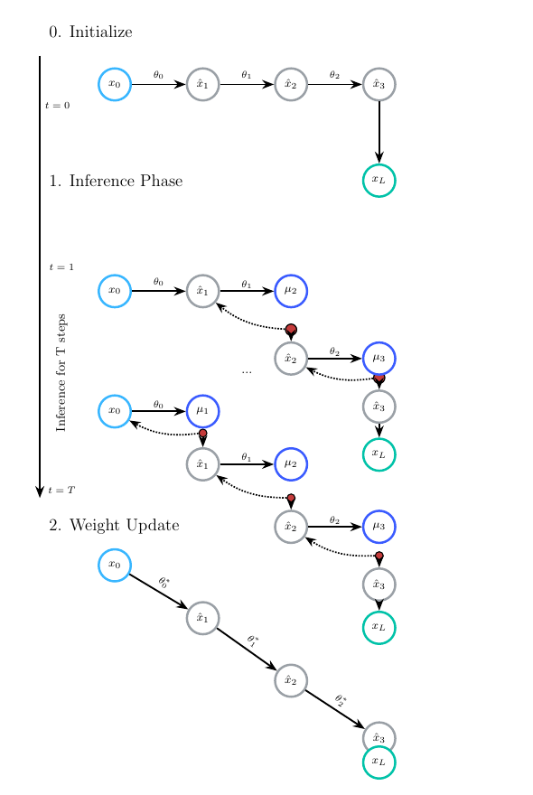
Figure 3: Inference Learning, the model clamps sensory input x_0 and supervision nodes x_L, infers latent states (gray) by minimizing prediction error (red), and only then performs a weight update.

Incremental Inference Learning (IPC)

Incremental PC (IPC) updates the weights at every time step of inference rather than waiting for full convergence. Intuitively this provides a continuum between standard PC's simultaneous convergence and BP's strictly phased updates, a continuous shift between PC and BP behavior. IPC tends to improve convergence speed and stability (weights are nudged gradually) and removes the need for an external control signal to switch phases, making it more autonomous and biologically plausible. On general non-layered networks it still does not exactly follow BP updates. Most baselines in this thesis use IPC.

PC on arbitrary graphs

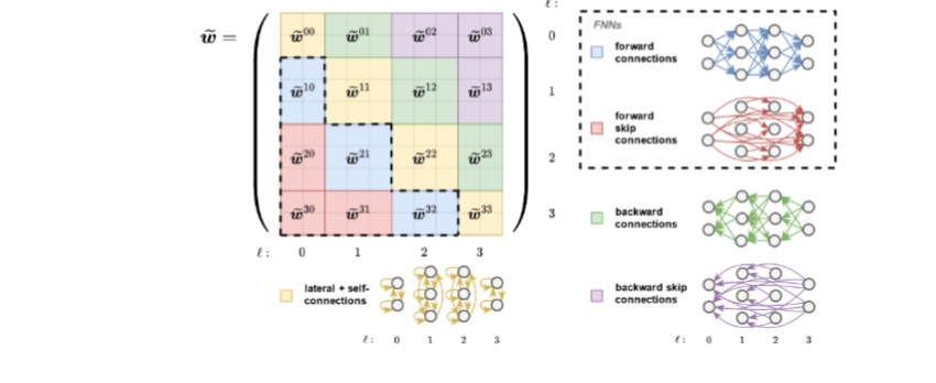
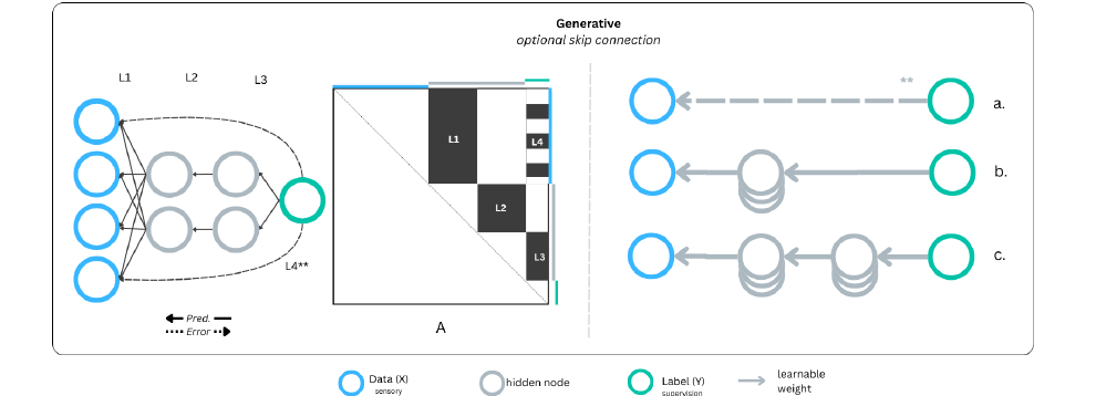
The central generalization: instead of a hierarchy of layers, consider an arbitrary directed graph G = (V, E). Following the ML convention, the adjacency matrix A is indexed with rows as targets (receivers) and columns as sources (senders), so W_ij is the weight on edge j → i (j predicts i). A subset of nodes are sensory nodes (external data), the rest are internal/latent nodes, and under supervision an additional subset is the label. Topology is no longer a chain, it is whatever the adjacency matrix encodes.

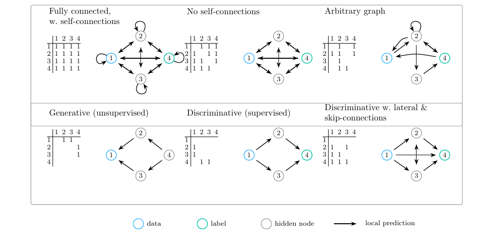
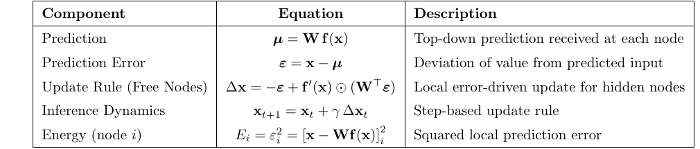
Figure 4: Different adjacency matrices and topologies — Figure 4: Different adjacency matrices determine the topology of the graph and therefore its learning dynamics, fully connected, no self-connections, generative, discriminative, and arbitrary graphs with lateral & skip connections.

At each step, node i computes a prediction µ_i from its incoming edges (typically a weighted sum through a nonlinearity f), and a prediction error ε_i = x_i − µ_i:

µ_i,t = Σ_j  W_ij f(x_j,t) = W f(x)
ε_i,t = x_i,t − µ_i,t

Training minimizes the total energy E_t = ½ Σ_i ε_i,t², the same free energy F rewritten as a sum over nodes instead of hierarchical layers. The inference (value) update and the Hebbian-like weight update are:

Δx_i  = γ ( −ε_i,t + f'(x_i,t) ⊙ (Wᵀ ε_t)_i )      # inference (E-step), weights fixed
ΔW_ij = α ( −ε_i,T  f(x_j,T) )                      # weight update (M-step)

Every derivative here involves only a node's direct neighbors, so updates are local in both implementation and time. PC and IPC are "1-hop in time": each update depends only on the present presynaptic activity and postsynaptic error, with no unrolling of the inference dynamics as temporal credit assignment (BPTT) would require.

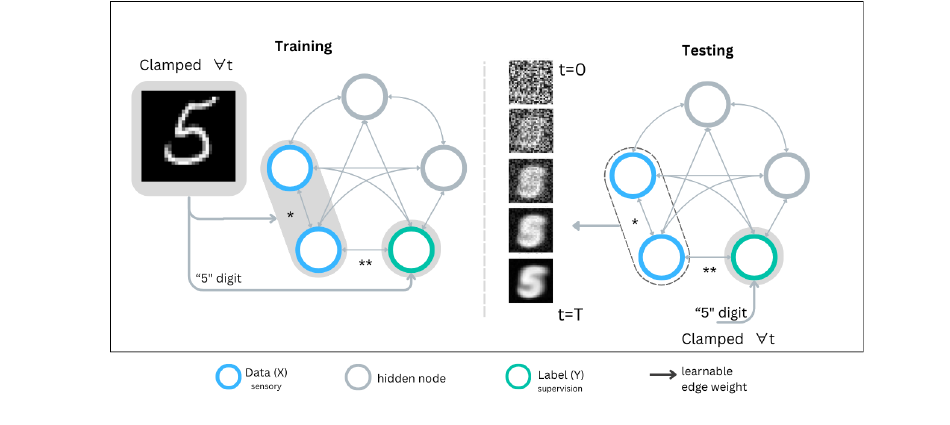
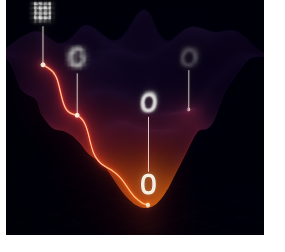
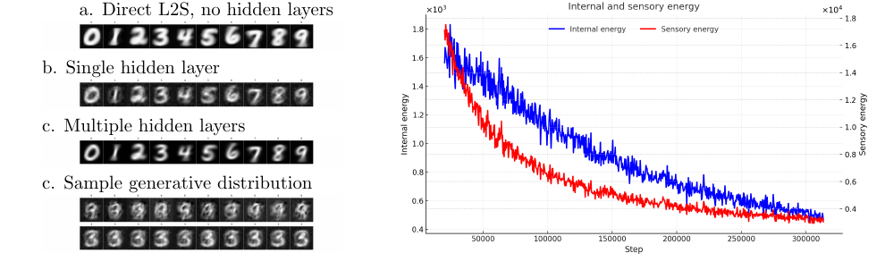
Figure 5: Training and testing of a fully connected graph — Figure 5: Training and testing a fully connected graph with sensory (gray), internal (white), and label (green) nodes, at test time we clamp either the sensory or label nodes, run inference to equilibrium, and recover the unclamped nodes for classification or generation.

Figure 6: Energy landscape shaped by inference and learning — Figure 6: Inference moves node values toward low-energy regions, while altering the weights shapes the energy landscape so that lower-energy states correspond to preferred (training-like) states.

Because the model is not trained on a single task, the same trained graph can be queried in different ways. Under query by conditioning, a subset of nodes is clamped throughout inference so the rest converge to the conditional expectation: clamp image pixels to infer the one-hot label (classification), or clamp a target label and start from a zero image to infer pixel intensities (generation). Reconstruction conditions on half an image (optionally plus the label) to infer the missing half.

Direction: reconciling two conventions

The neuroscience and ML literatures use opposite conventions for the local prediction. The thesis fixes this with one rule of thumb, predictions follow W; errors flow via Wᵀ, and shows the van Zwol (bottom-up, MLP-compatible) and Salvatori (top-down, generative) notations are reconciled by a single transpose, W^VanZwol = (W^Salvatori)ᵀ. The local equations are unchanged across classification and generation; only the boundary conditions (which nodes are clamped) differ. The thesis adopts the van Zwol convention: predictions travel from lower- to higher-index nodes, errors travel back down.

Figure 7: Fixing sensory and label nodes in the graph — Figure 7: Sensory nodes are fixed at the input (W⁰, images) and label-related weights are fixed at the output (Wᴺ); a block W^lk denotes weights from layer k sending predictions to layer l.

Architectures and tasks studied

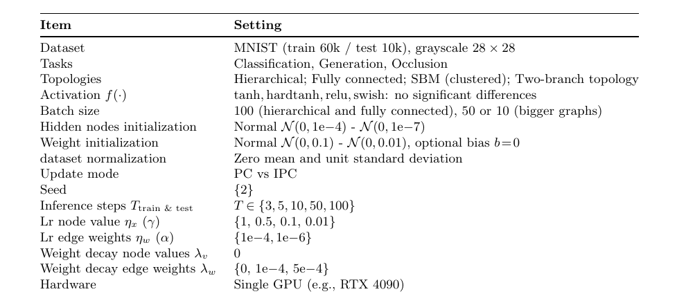
All experiments run on MNIST (784 = 28×28 sensory nodes, 10 supervision nodes for the one-hot digit), in PyTorch on a single RTX 4090, with both dense matrix-multiplication and torch-geometric message-passing implementations.

Discriminative PC

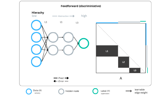
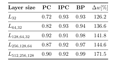
Here the graph learns a direct mapping X → Y; sensory nodes stay clamped through evaluation and the predicted class is read off the highest supervision-node values. Comparing PC, IPC, and BP across MLP-like architectures of increasing depth reveals a key finding: adding layers does not consistently help PC. The Δw metric, the normalized average absolute difference between IPC and BP weights, rises with depth (from ~126% to ~172%), indicating deeper PC models inject more noise into signal propagation and diverge further from BP's training dynamics.

Figure 8: Simplified MLP architecture trainable with BP or PC — Figure 8: A simplified MLP architecture that can be trained with either BP or PC, predictions and errors are stored in the nodes themselves, with prediction/error flow directions assigned for analogy.

Table 1: MLP accuracy under PC, IPC, BP across depths — Table 1: MLP architectures trained 15 epochs with PC, IPC, and BP (MNIST test accuracy, T_train = T_test = 35), Δw is the normalized average absolute difference between IPC and BP, which grows with depth.

Generative PC

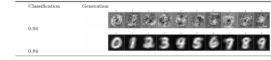
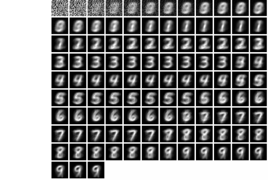
Generation runs the mapping in reverse: clamp the one-hot label, seed the sensory nodes with random noise, and use inference to fill in pixel intensities. This is intrinsically harder, MLPs handle spatial structure less efficiently than CNNs or VAEs, and the model has no direct control over output attributes. Sampling different digits of the same class by re-initializing the layer closest to the label produces little control and sometimes chaotic images.

Figure 10: MLP-like generative architecture under IPC — Figure 10: MLP-like hierarchical architecture trained with incremental PC, generating MNIST digits 0–9, with the energy plot of a generative model using hidden nodes L = {150, 100, 100}.

Fully connected (Hopfield-like)

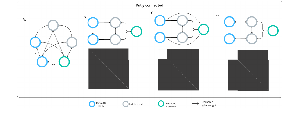
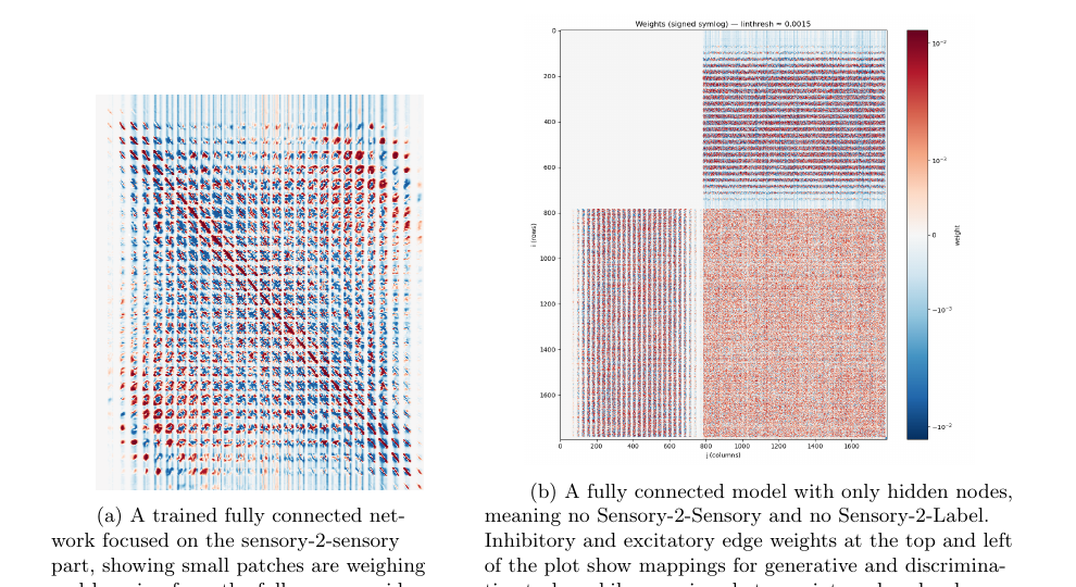
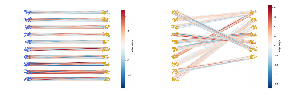
With no apparent hierarchy there is no top-down/bottom-up distinction; the model resembles a Hopfield/Boltzmann associative memory where the same node values serve both discriminative and generative tasks. The thesis probes the role of different edge types by selectively removing direct sensory↔label connections.

Try it: predictive coding as inference

To make this concrete, here is a tiny fully-connected predictive-coding network running live in your browser. Four prototype digits (0–3) are written into the weights with a single Hebbian rule (no training, no dataset). Clamp a label and watch the free pixel nodes settle, the network's energy descends as the prediction errors shrink, and the stored digit emerges. This is generation-by-inference, exactly the mechanism described above.

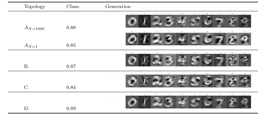
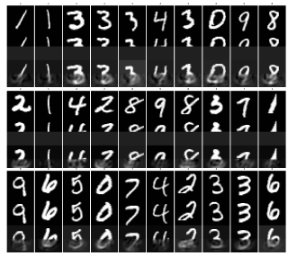
Table 2: Best stable IPC per topology — Table 2: Best stable IPC model (N = 1000) per topology, evaluated on classification (1000 MNIST test images) and digit generation, generation results were taken from epoch 1 due to instability.

Figure 12: Occlusion reconstruction with and without label — Figure 12: Occlusion/reconstruction, given half of the sensory image, the model infers the most likely missing half (and indirectly the class), with or without the label, much like an associative-memory task.

The fully connected model falls short of hierarchical networks trained with BP or IL, depth, which it lacks, appears empirically crucial. But it does demonstrate that one PC model can store an internal representation of a dataset and be queried to solve multiple classification and generation tasks reasonably well.

Initialization and convergence instability

PCNs can converge to correct solutions or settle in incorrect local minima. Too-large learning rates cause unstable inference and explosive values; too-small rates halt learning. The model can also collapse into a degenerate inverse representation (e.g. inverting black and white) that minimizes loss trivially. Prior convergence analysis shows sequential PCNs only converge under conditions, small initializations, small weights, and appropriate step sizes, with counterexamples where nonlinear dynamics and bifurcations cause non-stabilizing oscillations. Accordingly, weights are initialized from a small zero-mean Gaussian (or a small constant plus stochastic deviation) to keep early predictions similar and prevent destabilizing error spikes. IPC, though less efficient (an extra weight update each step), is more stable and yields better hierarchical performance.

Table 3: Unstable / partially collapsed fully connected IPC — Table 3: Best unstable or partially collapsed IPC (1000 internal nodes, S2S and S2L connections removed), by trading off learning rates and decay, the fully connected model can reach hierarchical-level classification at the expense of generation.

What the weights learn

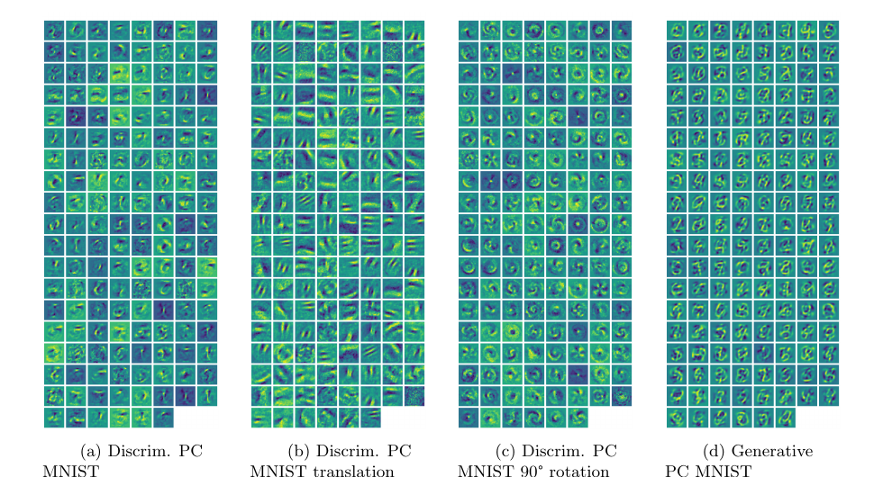
PCNs develop features comparable to those learned by BP, classical edge detectors and Gabor-like filters, and self-organize around the symmetries present in the data. Discriminative PC on standard MNIST learned CNN-like averaging filters; on translated digits it independently discovered the Fourier transform (which diagonalizes shifts); on rotated and scaled digits it learned a Gabor transform (a Fourier transform in log-polar coordinates, ideal for rotation and scaling), all without being told to.

Figure 13: Learned discriminative and generative PC weights — Figure 13: Learned weights, discriminative PC on standard, translated, and 90°-rotated MNIST (left) self-organizes into general features, alongside generative PC weights (right).

Try it: train a layered PC classifier

This second demo trains a small layered predictive-coding classifier (64→36→10) on real 8×8 digits, 0–9, live in your browser, no backprop, only the local PC update rule. Click Train and watch test accuracy climb while the input→hidden weights self-organize into digit features, exactly the effect shown in Figure 13. Then classify held-out digits or draw your own.

Figure 14: Fully connected weights showing little internal structure — Figure 14: In the fully connected model the lack of incentive for internal-to-internal communication yields little visible structure between hidden nodes, while sensory-to-sensory weights resemble a Boltzmann-machine correlation matrix.

Figure 15: Weight matrix with weight decay and value init — Figure 15: With weight decay (λ_w = 1e−4) and small value initialization, some internal structure can be imposed, but without improving classification or generation, suggesting these are random artifacts rather than dataset-driven structure.

The shortcut problem in fully connected graphs

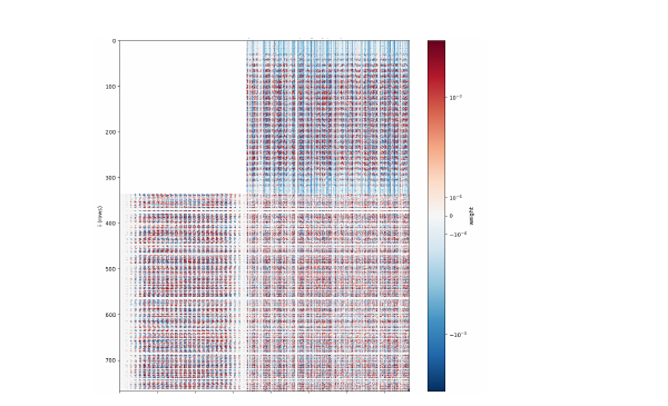
This is one of the thesis's central findings. When a fully connected graph includes direct sensory-to-label connections, energy minimization concentrates credit on the shortest error-reducing routes. The gradient on the sensory↔label blocks is large, rapidly driving a shallow one- or two-hop solution that bypasses most internal nodes. This is not a quirk of PC (or BP) but a consequence of the objective combined with a topology that permits shortcuts. Without constraints, the fully connected model collapses into two effective branches, a near-direct image→label map and a near-direct label→image map, and forms no compositional features in deeper assemblies. The result resembles a shallow associative link rather than a hierarchical representation, which is a problem because it is precisely the hidden layers that learn the intrinsic, generalizable features.

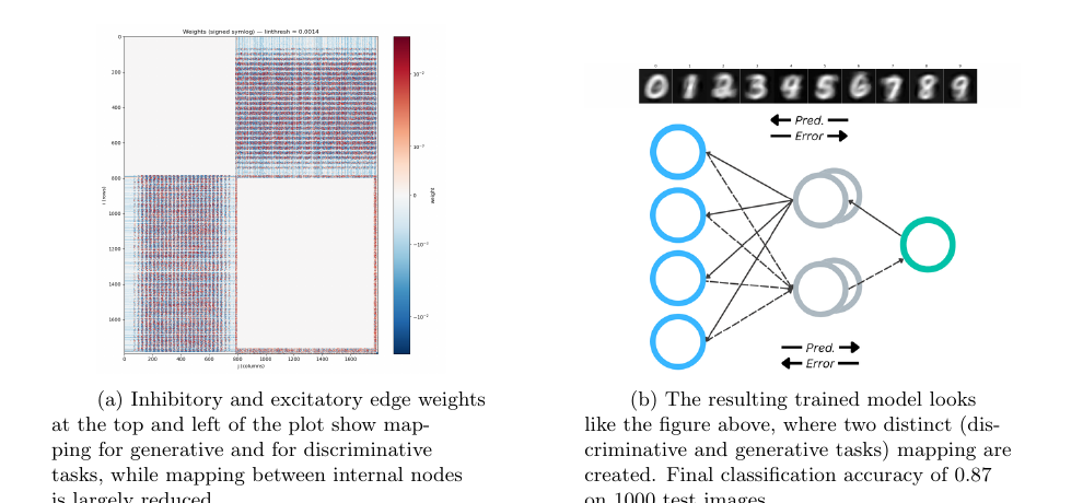
Figure 16: Forcing communication through 10 internal nodes — Figure 16: Starting from a fully connected graph and removing all but 10 internal nodes forces communication through them, yielding two distinct discriminative/generative mappings and 0.87 classification accuracy on 1000 test images.

One escape route (from work on causal inference) presupposes the graph and infers it from data: a fully connected x → y mapping underfits, so the model spontaneously inserts latent nodes and removes direct input-output edges, organizing a two-layer hierarchy that both minimizes free energy and halves the test error, driven by sparsity and acyclicity penalties in the loss.

Stabilization and scalability

A major strength of PC is that each layer's computation, forward and backward, is local and therefore parallelizable, removing one of BP's main bottlenecks on deep networks. In principle PC should scale well on large, sparse graphs with a message-passing implementation. In practice it is hard to scale due to model collapse and weak local error propagation as depth grows. The thesis attacks this from two directions: optimizer-level generalization tricks, and better graph structures.

Fast and slow updates, and Grokfast

Inference and learning naturally occur at different rates (different learning rates lr_x and lr_w, reflecting T inference steps per weight update). This motivates fast/slow learning ideas: fast plasticity for real-time adaptation, slow plasticity for long-term consolidation, echoing biological timescale hierarchies (faster sensory areas, slower higher-order areas) and the spectral asymmetry of ascending gamma-band prediction errors vs descending alpha/beta predictions. Grokfast amplifies the slow-varying (low-frequency) component of the parameter gradients via an exponential moving average, on the theory that slow-varying parameters drive generalization (the delayed-generalization "grokking" phenomenon).

Grokfast-EMA gradient amplification:
  ḡ_t = α · ḡ_{t-1} + (1 − α) · g_t      # EMA of gradients
  g'_t = g_t + λ · ḡ_t                    # amplify slow component
  W_{t+1} = W_t − η · g'_t

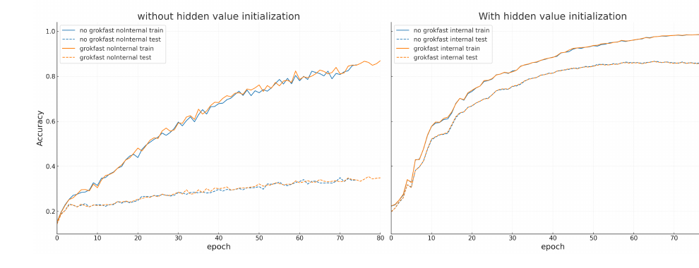
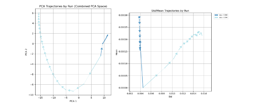
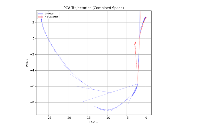
In this setting, Grokfast did not induce delayed generalization in the discriminative IPC model, test accuracy stagnated even after 150 epochs. Interestingly, training and validation accuracy rose in parallel when hidden values were randomly initialized before inference, suggesting the optimizer and inference dynamics already stabilize learning without gradient amplification. For fully connected models, Grokfast's effect was negligible, the fully connected starting topology was itself the bottleneck.

Figure 17: Grokfast does not improve test accuracy — Figure 17: Discriminative IPC trained on 1000 samples, Grokfast alone does not improve test accuracy.

Graph topology: DisGen, SBM, and scaling

The model's expressiveness is bounded by the message-passing scheme and the graph architecture. The shortest path between sensory node x and supervision node y must fall within T hops, so a small T constrains learning to short-range connections. The thesis then explores topologies that discourage shortcuts while promoting feature learning.

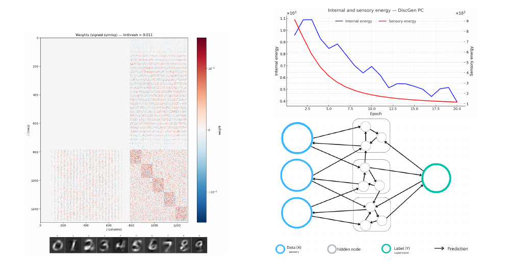
DisGen PC combines a discriminative and a generative branch (each two dense layers of {150, 50} nodes) with no lateral links between them, effectively two smaller models trained at once. Because the branches need different initial parameters, the combined model underperforms the individual ones.

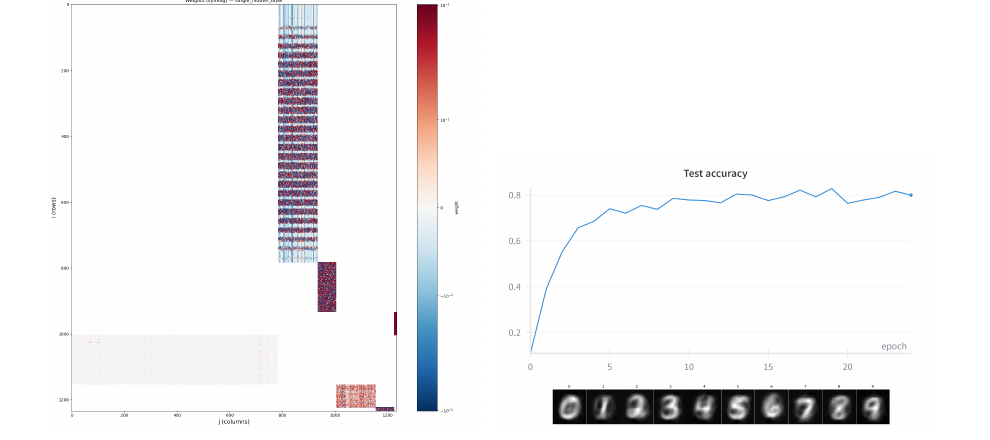
Figure 18: DisGen PC model with two branches — Figure 18: The DisGen PC model with two branches of L = {150, 50} internal nodes (T_train = T_test = 100); after training, most weight mass concentrates in the generative branch.

Random SBM. Inspired by weighted stochastic block models used as priors for the human connectome, the graph is treated as a directed SBM with one sensory block, K equal-sized internal communities, and a supervision block, with edges sampled at intra-community probability p_intra and inter-community probability p_inter, trading density inside communities against clustered sparsity between them. With p_intra = 0.25, p_inter = 0.1, and 5 clusters of 100 internals, classification reached 0.81. Pushing internal nodes to 6000 improved classification but degraded generation, echoing the fully connected case.

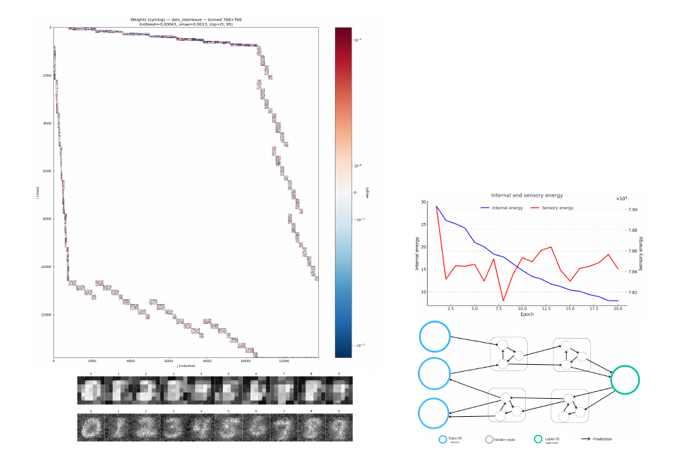
Figure 19: Random SBM PC model — Figure 19: The random SBM PC model with five internal clusters of 100 nodes each, its generative evaluation, and the internal/sensory energy over training.

Two-way layered SBM. To scale while preventing shortcut mappings, branches are initialized layer by layer with an imposed hierarchy: a discriminative branch (x → H → y) and a generative branch (x ← H ← y). Each "layer" is itself a stochastic block rather than a dense layer, with inter-layer wiring set by p_inter for tunable modularity; MNIST pixels enter as overlapping/non-overlapping 4×4 patches that are pooled into successive layers. This design lets you scale depth, width, and clustering while tuning sparsity. The largest experiment used ~14,000 nodes and over 2 million edges, and crucially, scaling the sparse topology up did not hurt classification (test accuracy ~0.78), confirming clustered sparse graphs scale without accuracy loss.

Figure 20: SBM model with 14k nodes and 2M edges — Figure 20: Graph topology of the SBM model with 14k nodes and over 2 million edges, generative granularity depends on the number of first-layer clusters, and a 0.78 test accuracy shows scaling the sparse topology does not degrade classification.

Try it: explore a two-way layered SBM

This playground runs a deliberately tiny version of the topology above (about 52 nodes instead of 14k), so it trains live in your browser. A 4x4 sensory block feeds a discriminative branch (x → H → y) and a generative branch (x ← H ← y), each built from sparse stochastic blocks (dense within a cluster, sparse between). Pick an input, hit Train, and watch the internal nodes settle by inference, the label nodes pick a class, and the PC energy fall as the local weight rule learns (no backprop).

Conclusion

The thesis formalizes PC on arbitrary directed graphs, reconciles the top-down and bottom-up notations, and derives local inference and weight-update rules needing only neighborhood information, unifying IL and IPC as a single energy-minimization process that can be instantiated across many topologies and queried for multiple tasks. The headline findings, restricted to MNIST:

• Shallow hierarchical PC/IPC reaches competitive classification accuracy, but simply adding depth does not reliably help, deeper stacks increase divergence from BP (larger Δw), with noisier error propagation and less stable training.
• The same graphs work generatively by clamping labels and inferring pixels, producing plausible digits but with limited controllability and fragile, hyperparameter-sensitive dynamics.
• Learned representations are nonetheless meaningful: PC self-organizes around task symmetries (Fourier/Gabor transforms under translation/rotation), much like BP.
• In fully connected graphs a single model can both classify and generate, but credit flows through the shortest paths, encouraging near-direct mappings that bypass richer internal structure.
• Clustered sparse topologies (SBM) discourage these shortcuts and scale to ~14k nodes / 2M edges without accuracy loss.

BP is largely confined to feedforward (and recurrent) structures for stable operation. PC, by contrast, can train arbitrary graphs and serve multiple tasks or modalities in one network, a potential path toward more brain-like connectivity (recurrent loops, multi-sensory integration) that BP would struggle with. PC is not merely a quirky approximation to BP: it trades exact global gradients for biological plausibility, parallel activity/weight updates, and cyclic multi-functional graphs, while remaining sensitive to initialization and step sizes.

Limitations & future work

All results are MNIST-scale, and PC/IPC training is sensitive to initialization, step sizes, and the number of inference steps T. The way forward is not to force PC into matching BP gradients exactly, but to pair it with topology and objectives that exploit its strengths, connectome-inspired priors, regularizers pushing the graph toward sparse layered substructure, penalties disfavoring shortcut edges, and skip-connected designs that keep effective credit paths short. Concrete directions include: (1) initializing or regularizing PC graphs with connectome data (à la continuous-state Hopfield networks set from functional connectivity); (2) altering the loss with ℓ2 weight decay or power-law (scale-free) degree regularization to encourage hub structure and hierarchy; and (3) dynamical graphs that grow connections where local error is high (NEAT/GradMAX/Firefly-style) and prune unused parts, learning topology directly from data (e.g. NOTEARS for DAGs).

Implementation & reproducibility

All models, discriminative, generative, fully connected, SBM, and two-branch, were implemented in PyTorch with both dense matrix-multiplication and torch-geometric message-passing dynamics, run on a single RTX 4090 with fixed seeds. Dense formulations compute over the full W matrix (scaling as N²), while message passing restricts computation to stored edges (scaling as |E|), far better reflecting PC's locality and suiting sparse, non-layered topologies. Unlike GNNs, which update node embeddings by neighborhood aggregation, PC updates node values by minimizing energy via local error feedback, nodes encode predictions and errors, not similarity-based embeddings.

Table 7: General training configuration, MNIST 28×28, classification/generation/occlusion tasks, hierarchical/fully connected/SBM/two-branch topologies, with the full sweep of learning rates, weight decay, inference steps T, and hardware.

Appendix highlights

The appendix expands the BP-vs-PC comparison, the neural inference simulations, and the parameter sweeps that underpin the main results.

BP vs PC, side by side

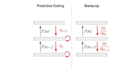
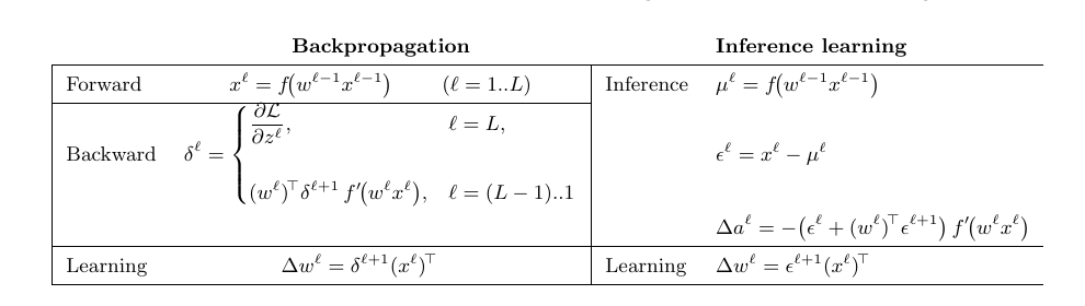
BP is a synchronous two-phase procedure with non-local, globally-coupled weight updates that must cache forward activations; PC uses an iterative, unified inference-and-learning process with strictly local (Hebbian-like) rules, no separate global gradient tape, and natural support for asynchronous/parallel updates. PC can approximate BP under conditions, converged inference on a DAG, feedforward initialization, low feedback precision, or locally linear activations, and BP-equivalent variants like Zero-Divergence Inference Learning (Z-IL) reproduce BP's exact weight changes using only local error units, with IPC sitting on the continuum between them.

Figure 21: PC vs BP update procedures — Figure 21: PC first runs iterative error minimization before a weight update based on inter-layer prediction errors, whereas BP propagates gradients backward in a dedicated backward phase and then updates weights directly.

Table 6: BP vs IL update equations — Table 6: A side-by-side comparison of the forward, backward/inference, and learning update equations for backpropagation and inference learning on a sequential model.

Figure 22: Stage-wise training in hierarchical PCN — Figure 22: Stage-wise (sequential) training in a hierarchical PCN, which distributes prediction errors more evenly across layers and improves gradient flow.

Neural inference dynamics

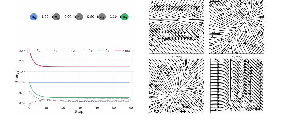
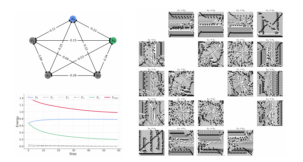
To study PC under controlled conditions, the thesis simulates inference as ODEs in continuous time on two toy graphs, a feedforward MLP-like chain and a fully connected network, with only the sensory (x₀ = 1) and label (x₄ = −1) nodes clamped and the hidden nodes free to minimize local error under f(x) = tanh(x).

Table 4: Key vectorized PC dynamics equations — Table 4: The key vectorized equations for PC inference dynamics, prediction µ = W f(x), error ε = x − µ, the free-node update, the step-based inference rule, and the per-node energy.

Figure 23: MLP-like model dynamics and vector fields — Figure 23: MLP-like model, its graph topology and inference energy (left) and the streamplot vector fields for each active edge (right), which converge to a single attractor.

Figure 24: Fully connected network dynamics — Figure 24: A fully connected PC network with symmetric weights and clamped endpoints, its all-to-all topology, the per-node and total energies (showing transient instability before convergence), and the richer pairwise vector fields.

Parameter sensitivity

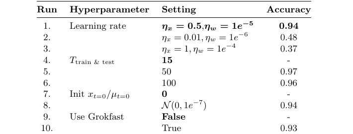
A systematic sweep over the discriminative IPC model confirms how sensitive PC is to its hyperparameters, above all the ratio between the two learning rates and the number of inference steps T. A balanced setting (η_x = 0.5, η_w = 1e−5) reaches 0.94, while mismatched rates collapse accuracy to 0.48 or 0.37; raising T from 15 to 50 lifts accuracy to 0.97.

Table 5: Discriminative IPC hyperparameter sweep — Table 5: Per-experiment training configuration and accuracy for the discriminative IPC baseline (hidden layers {300, 100}, swish), each row varying a single hyperparameter from the baseline.

Figure 25: Effect of weight decay on generation — Figure 25: The effect of weight-decay values on generative output, sequential generative PC produces sensible images even with zero weight decay (λ_w = λ_x = 0).

Figure 26: PCA and std/mean weight trajectories — Figure 26: PCA trajectories and standard-deviation/mean weight trajectories of the two fully connected models from Table 3, revealing different training dynamics from the same initialization.

Figure 27: PCA weight dynamics under Grokfast — Figure 27: Weight dynamics of several fully connected IPC models via PCA (one arrow per epoch), Grokfast appears as damping in the trajectory, but classification accuracy does not improve.

Figure 28: Transitioning from noise to digits by altering the label — Figure 28: Transitioning from noise to increasingly clear digits by altering the clamped label.

Figure 29: Generation with the label clamped to 5 — Figure 29: Image generation with the supervision labels clamped to the one-hot encoding of the digit 5.

Figure 30: Reconstruction on rotated and scaled data — Figure 30: Reconstruction experiments where the dataset has been rotated or scaled.

Figure 31: Illustration of the SBM models, sensory nodes (blue) form clusters each mapping a 4×4 patch, with hidden clusters wired fully or directionally depending on the SBM topology type.

Keywords: predictive coding, inference-learning, graph topology